Chris. Bart.

May I use Proton?

... with birds visiting and gliding effortlessly through the air

Post a pic you took, no context, to bring some zen to the feed.

Confidence intervals with maximal average power We propose a frequentist testing procedure that maintains a defined coverage and is optimal in the sense that it gives maximal power to detect deviations from a null hypothesis when the alternative to...

Bookmarked. Need to read carefully.

FYI, The figure is very similar to arxiv.org/abs/1905.03981, in which we use repeated sampling from hypothesis, and assess the use of priors for frequentist confidence intervals.

DAG representing the causal structure of a standard difference-in-differences design with two locations and two time periods—units in one location in the post-period receive treatment. $L$ = group or location indicator (treated vs. untreated location); $T$ = time indicator (pre vs. post period); $U$ = unobserved time-invariant confounders (e.g., GDP per capita, general health status, public health infrastructure). $X \leftarrow T \rightarrow Y$ represents a common time trend affecting both locations equally. The causal effect of $X$ on $Y$ is identified by conditioning on $\{L, T\}$, which corresponds to using location and time indicator variables in a regression like `y ~ location * period`.

DAG representing the causal structure of a standard difference-in-differences design, but with explicit pre- and post-treatment outcomes. $L$ = group or location indicator (treated vs. untreated location); $T_\text{post}$ = post-period measurement (indicator that the observation occurs after the intervention); $X_\text{post}$ = treatment (which only occurs for treated locations in the post period); $Y_\text{pre}$ and $Y_\text{post}$ = outcome measured before and after the intervention. $U$ = unobserved time-invariant confounders (e.g., GDP per capita, general health status, public health infrastructure). $Y_\text{pre} \rightarrow Y_\text{post}$ represents outcome persistence (e.g. autocorrelation or slow-moving changes); $X_\text{post} \leftarrow T_\text{post} \rightarrow Y_\text{post}$ represents a common time trend affecting both locations equally. The causal effect of $X_\text{post}$ on $Y_\text{post}$ is identified by conditioning on $\{L, T_\text{post}\}$, which corresponds to using location and time indicator variables in a regression like `y ~ location * period`.

spending my sunday evening once again attempting to draw a DAG for diff-in-diff

📣The 2026 Symposium of #CausalInference in the #HealthSciences takes place on March 18, 2026 in Fribourg. Theme: AI & machine learning in causal inference for health sciences
🎤Keynotes: Elsa Gautrain, Aurélien Sallin, Jonas Peters, Jana Mareckova
🔗https://projects.unifr.ch/pophealthlab/?page_id=1561

Some Common Dose–Exposure–Response Estimands and Conditions for Their Causal Identifiability Exposure–response analyses are central to dose selection in drug development. The estimand framework, formalized in ICH E9(R1) regulatory guidance, provides a structured approach to define scientific...

We apply the estimand framework to dose–exposure–response analyses. ... strategy to improve exposure–response analyses for dose selection, particularly when the relevant evidence includes data from multiple studies.

#estimand #exposure-response #dose-response #causal

doi.org/10.1002/psp4...

Confidence Regions for Multiple Outcomes, Effect Modifiers, and Other Multiple Comparisons In epidemiology, some have argued that multiple comparison corrections are not necessary as there is rarely interest in the universal null hypothesis. From a parameter estimation perspective, epidemio...

For years I had trouble following some of the discussion about confidence bands, but at ACIC this year @noahgreifer.bsky.social pointed me to a helpful paper

So you don't have to be as perplexed as I once was, we have a new pre-print introducing the key ideas
arxiv.org/abs/2510.07076

adrftools: Estimating, Visualizing, and Testing Average Dose-Response Functions Facilitates estimating, visualizing, and testing average dose-response functions (ADRFs) for characterizing the causal effect of a continuous (i.e., non-discrete) treatment or exposure. Includes suppo...

I'm so excited to announce the first release of my newest #Rstats package, {adrftools}! This package facilitates estimation, visualization, and testing for the causal effect of a continuous (i.e., non-discrete) treatment.

🧵 1/10

#statssky #episky #causalinference

Thanks for these posts. I would have answered that live would be boring if you can only analyze pre-registered compliant data.

Your answer makes much more sense.

👏

As I said, this is the important work that needs to be done. Mark's paper is overly simplistic, arguing we can't judge deviations at all. Deviations are in practice not remotely as bad as he wants. If he had collected actual data,che would have falsified his own claims.

Here an example of using DAG/SWIG to assess a situation with an underlying process that is continuous in time, and interventions and observations that are discrete.

bsky.app/profile/chri...

Ok ... if the data is a sample from a larger population, then it may be convenient to describe the relation between the two via a distribution from which the data is sampled.

Ok ... the functional form by which the independent variables affect the dependent variable matters. When you use linear models as a tool, you may have to transform the independent variables.

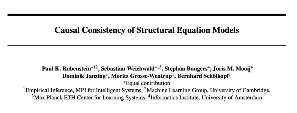
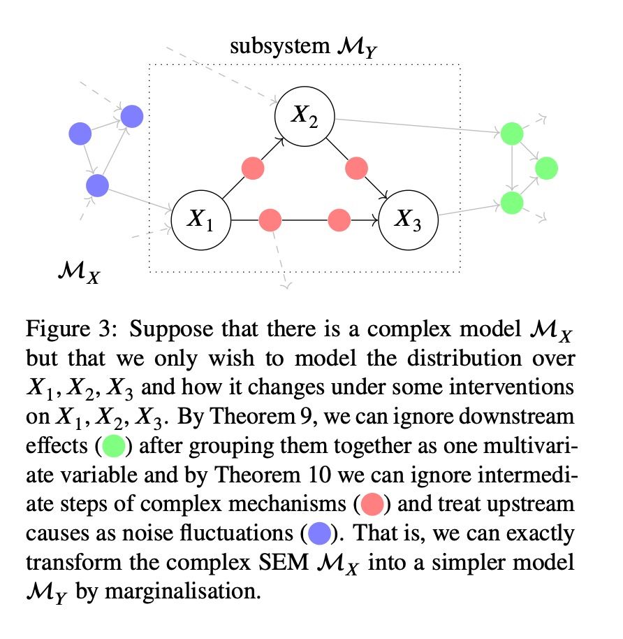
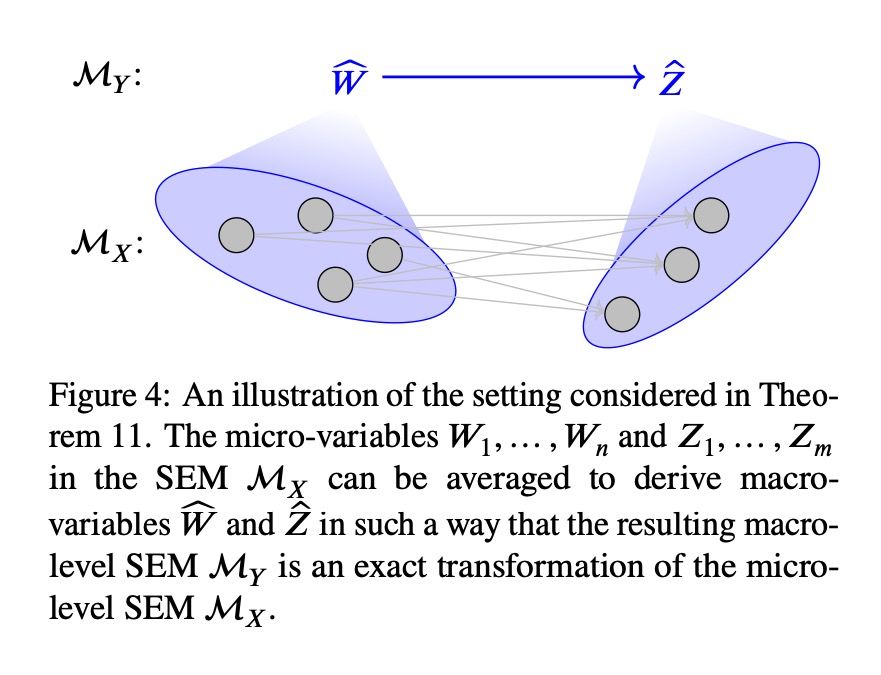
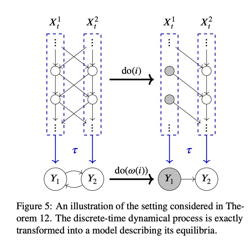
This is a fairly technical but highly relevant paper on how we can model complex systems at various levels of detail without losing causal content. Think gas: instead of tracking every molecule, we can focus on big-picture properties like temperature and pressure. www.auai.org/uai2017/proc...

Question that intrigued me a lot. My current view:

Arrows can represent the process that is continuous in time. Edges are values of the process at selected time points of particular interest.

We have to be careful. Sometimes, a data summary may nonetheless answer a different question, and this different question could be of interest.

Don't do anything since there might be a bias might be counterproductive!

Why it matters
1️⃣ Clear estimand definition – the target of inference is stated up front, removing ambiguity.
2️⃣ Transparent causal assumptions – DAGs & SWIGs show which confounding paths are blocked.
3️⃣ Step‑by‑step DER derivation – fits into the standard dose‑exposure‑response workflow.

2/6

What are some of the best DAGs you seen that depict time-varying confounding?

Could be from a 'real' worked example, or generic.

#EpiSky

Or as joint outcomes? With the mediator helping to explain variability of the outcome?

We propose a method for estimating long-term treatment effects with many short-term proxy outcomes: a central challenge when experimenting on digital platforms. We formalize this challenge as a latent variable problem where observed proxies are noisy measures of a low-dimensional set of unobserved surrogates that mediate treatment effects. Through theoretical analysis and simulations, we demonstrate that regularized regression methods substantially outperform naive proxy selection. We show in particular that the bias of Ridge regression decreases as more proxies are added, with closed-form expressions for the bias-variance tradeoff. We illustrate our method with an empirical application to the California GAIN experiment.

arXiv📈🤖
Long-Term Causal Inference with Many Noisy Proxies
By Lal, Imbens, Hull

Uruguay’s Renewable Charge: A Small Nation, A Big Lesson For The World Uruguay built a power grid that runs 99% on renewables—at half the cost of fossil fuels. Here’s how its bold energy overhaul became a global model.

“Uruguay did what most nations still call impossible: it built a power grid that runs almost entirely on renewables—at half the cost of fossil fuels. The physicist who led that transformation says the same playbook could work anywhere—if governments have the courage to change the rules.”

X/Twitter's rough full volume is around 500 total million posts every day, or 182 (and a half) billion posts per year.

By contracts, we found 11.2 million research posts in all of 2025 on there.

In other words, 0.000006% of Twitter appears to be sharing research. Basically zero.

This gives financial institutions leeway to acquire hard-to-sell, higher-yielding long-term assets and finance them with cheaper short-term liabilities, thus increasing profits through a risky “mismatched book”.

link 📈🤖
Demystifying Proximal Causal Inference (Ringlein, Nguyen, Zandi et al) Proximal causal inference (PCI) has emerged as a promising framework for identifying and estimating causal effects in the presence of unobserved confounders. While many traditional causal inference methods rely on the

Enjoy two weeks of Proton for free Experience true online privacy. Protect your data with Proton for free for the next 14 days.

Happy new year! As an idea for improved privacy pr.tn/ref/X11M0Y8Q

Lumo rendering an integral in LaTeX.

Lumo now understands LaTeX. Type any formula (fractions, matrices, integrals, etc.) straight into chat and see it rendered instantly. No more screenshots or ASCII tricks. Perfect for precise technical work and academic tasks.

Try it now: https://lumo.proton.me

Students learn early that correlation does not imply causation. Correct, but incomplete... Certain patterns of independence and conditional dependence constrain #causal structure very strongly. A simple example:

The older I get, the more my politics mature from childish, naïve beliefs like "the world is complicated and leaders have to make hard decisions" to more serious, adult principles like "hurting people is bad and helping people is good."